|
Step 1: Launch Maple. Starting Maple interface
looks like the images below.
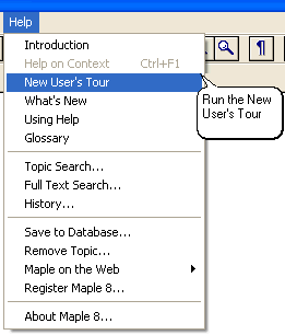
Click on Help and select
New User's Tour.
Then at the bottom of the new page select
Click here to begin the New User's Tour
Step 2: In the new page, Maple New User's Tour -
Main Menu, there are twelve topics that you can choose from. I recommend that you go
through them in order to make yourself familiar with Maple interface. So check items 1
(Working Through the New User's Tour), 2 (
The Worksheet Environment), 3 (Numerical Calculations),
and 4 (Algebraic Computations) before continuing to the next step.
Step 3: Click on number 5 (
Graphics). Maple can plot both 2-D and 3-D graphics which by default would
appear as inline graphics just under the commands in the worksheet. As stated in the page,
"Related functions (such as plots) in Maple are grouped into packages and
can be accessed by using the notation package[function](arguments)." To
see what commands are available in the plots package, use the
with command.[> with(plots);
and press enter while the cursor is anywhere in that field. A list of the functions
available in the package will be displayed similar to the list below:
animate, animate3d, animatecurve, arrow, changecoords,
complexplot, complexplot3d, conformal, conformal3d, contourplot,
contourplot3d, coordplot, coordplot3d, cylinderplot,
densityplot, display, display3d, fieldplot, fieldplot3d,
gradplot, gradplot3d, graphplot3d, implicitplot,
implicitplot3d, inequal, interactive, listcontplot,
listcontplot3d, listdensityplot, listplot, listplot3d,
loglogplot, logplot, matrixplot, odeplot, pareto, plotcompare,
pointplot, pointplot3d, polarplot, polygonplot, polygonplot3d,
polyhedra_supported, polyhedraplot, replot, rootlocus,
semilogplot, setoptions, setoptions3d, spacecurve,
sparsematrixplot, sphereplot, surfdata, textplot, textplot3d,
tubeplot
representing a wealth of options available to the user.
Step 4: Creating plots in Maple is really
easy and as you get to practice and explore your options, you will develop an understanding
of how to manipulate the commands, the resulting plots will look better and better. Let's
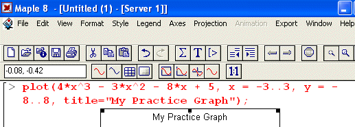
start with a 2-D function of y = 4 x3 - 3 x2
- 8 x + 5. We need to define a set of values for x for which
we would calculate the associated values for y. This is done by x = -3..3 and
y = - 8..8, which is indicating that values of x would range between -3 to
+3 and y between -8 and +8. These are the starting values and we
can adjust them after we see the actual plot (Of course you may choose to substitute
x = - 3 and x = + 3 in the function and find the actual y values
associated with the range, if you choose to do so). We can also put a title for the plot by
simply adding title="My Practice Graph" to the arguments of the command.
Finally the plot command for our function is:
[>plot(4*x^3-3*x^2-8*x + 5, x =-3..3, y =- 8..8, title="My
Practice Graph");
Press Enter and you should get the following plot.

If you click once inside the plot, the object handles will appear that would allow you
to resize the object similar to what you do in any word processor. Also notice that as
you click on plot area besides the handles you will also see new options added
to the text toolbar. (Compare it with the image in Step 1)
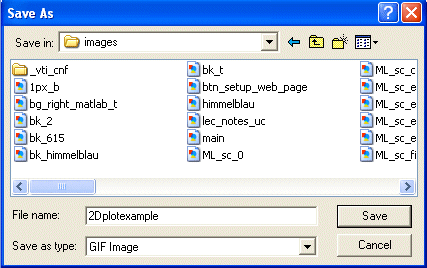
Select Export and one of the graphic formats such as GIF.
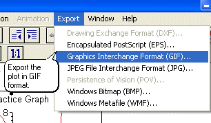
A standard Save As window opens where you may save the graph at a desired location.
This image can now be used in any Web page and or word processor and can be edited and modified
with any graphic software such as Paint Shop Pro.
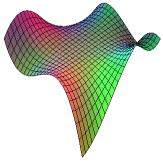
Step 5: Creating 3D plots is also very
easy. The procedure is similar to the ones in Step 4 with a couple of
additional information to be supplied to the plot command which in this case is
plot3d. Let's assume that we want to plot the 3-D function of
z = 4 x3y - 3 x2y2 - 8 xy3 + 10.
We need to define a set of values for x
and y for which
we would calculate the associated values for z. We can also modify the display of the
graphics by changing fonts, lighting, coloring and more. Again we need to define the range
for x and y which we do by x = -3..3 and y = - 3..3. As
before, these are the starting values and we can adjust them after we see the actual plot.
Add a title for the plot, title="My 3D Graph", and lights, lightmodel=light1 to the
arguments of the command. Finally the plot3d command for our function is:
[> plot3d(4* x^3*y-3*x^2*y^2-8*x*y^3+10, x=-3..3,
y=-3..3, lightmodel=light1, title="My 3D Graph" );
Press Enter and you should get the following plot.
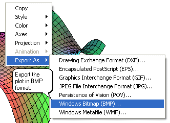
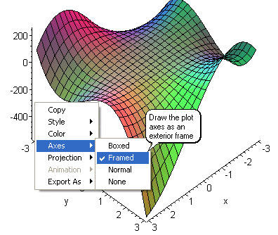
As before, we can click the image once and when the handles appear modify the image presentation.
For example, we can save the image as described in Step 4. But this time let's do it in a
different way. First, press and hold the left mouse button anywhere inside the handle box and move
the mouse to left, right, up, and down. You will notice that plot will rotate along its axes,
depending on which direction the mouse moves. That is how you can rotate a plot to examine its
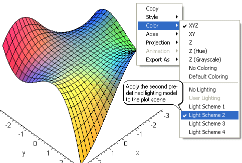
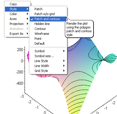
local and global maximum and minimum points. Now right-click anywhere inside the box.
A window will pop up that will allow you to modify the graph presentation. Below are few options
that can help you save the image, place axes, lights, colors, and so on.
To further explore the
capabilities of Maple, use the help menu.
Additional tutorials related
to our topics will be available soon.
|