
Random Number Generation
There are several methods that deal with generating successive random samples from a probability
distribution. All these methods are based on the use of
![]()
![]() random numbers. We will
discuss several methods and list a number of algorithms to generate random numbers. Three
general approaches are:
random numbers. We will
discuss several methods and list a number of algorithms to generate random numbers. Three
general approaches are:
Inverse Method
The inverse method is based on the property that the values of the cumulative distribution functionExamplecan be considered as samples from
. To obtain a random sample
from the probability density function
, we first determine the cumulative distribution function
. Since,


, we generate
and solve


. So, the random sample will be:
It is easy to recognize that when

F -1(
)
is not in closed form, or when


can not be easily solved, then this method should not be used.
Generating a random sample fromConvolution Method(
,
).
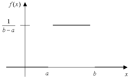
Probability density function for the Uniform distribution is given by:


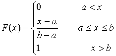
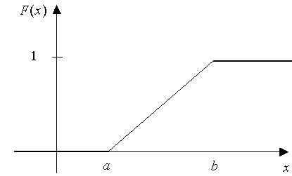
The cumulative distribution function for this distribution is given by:


Setting
=
, then
= F -1(
) = (


)
+
.
The basic idea of this method is to use special properties of some distributions and express the distribution as the statistical sum of other easy to sample random variables. Usually easy to sample refers to those distributions which Inverse Method can be applied to them. Erlang and Poisson distributions are typical examples of the distributions to which the Convolution Method can be applied. In both cases the easy to sample distribution is the exponential distribution.Example
Generating a random sample from m-Erlang(Acceptance-Rejection Method)
m-Erlang(
) random variable
is defined as the statistical sum of m
exponential (
) random variables. Let
be the m-Erlang(
) random variable, then
where


,
, . . . ,
's are
exp (
) random variables.
Each
can be generated using the the Inverse method by


(
). So,


{
(
)

(
)
...

(
)}


{
(

...
)}
This method is designed for random variables with complex probability density functions,, where the Inverse or Convolution methods are not generally applicable. In this method, we replace the complex probability density function
with a more analytically manageable proxy
,
. We then generate samples from
and use them to determine samples from
.
To determine
, we first define a majorizing function
such that it dominates
in its entire range. That is
Next, we define the proxy


of
by normalizing
as:
Note that the denominator in the above formula is actually the area under the

curve.
Now:
The less rejection in Step 4, the more efficient this method is. That in fact depends on how close the majorizing function
- Define
and determine

- Generate a random number
from
using the Inverse or Convolution method
- Generate
. [Remember that this
is different from any
that you have generated in step 2]
- If


/
then accept
as a random number from
, otherwise reject it and go to Step 2.
is defined to the actual
.
Example
Generating a random sample from beta (,
)
Probability density function for the beta is:
where

is the beta function defined by:
So, beta (

,
)
12
(


) for


, and
at other places. This function at the (
,
) interval has a maximum at


, with

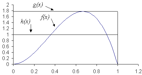
16/9. Therefore,

16/9 majorizes
at the above interval. Computing the proxy
of
distribution function we will have


/[area under
]
(16/9)/(16/9)

. All three functions are depicted in the following graph.
To see how the algorithm actually works, assume we generated


0.3135.
Using this value ofwe will generate

0.3135 from
. (Remember that

1, so,


by inverse method).
We now generate anotherand compare with the ratio that we just calculated. Assume

0.7803
We then calculate:
g(0.3135)16/9
1.77778,
f(0.3135)12(0.3135)2(1-0.3135)
0.80965 and
/

g(0.3135)/f(0.3135)
0.80965 / 1.77778
0.45543.
since 0.7803 > 0.45543 we reject this sample and continue by repeating the algorithm again.
Here are procedures for generating random numbers from well-known distributions:
Discrete Random Variables
Bernoulli
(![]() )
)
- Generate

- If


 ,
set
,
set


 ,
,
otherwise,


Discrete Uniform
- Generate

- Set

 I
I

 (
j
(
j  I
I

 )
)


Binomial
(t,![]() )
)
- Generate
 ,
,
 , … ,
, … ,
 as
as
 Bernoulli
(
 )
random variables
- Set


 …
…


Geometric
- Generate

-


Negative Binomial
(s,![]() )
)
- Generate
 ,
,
 , … ,
, … ,
 as
as
 Geom (
 ) random
variables
- Set
 =
=


 …
…


Poisson
![]()
- Let


 ,
,


 , and
, and

 0
0
- Generate

 , and
replace
 by
by


- If


 , set
, set


 . Otherwise, replace
 by
by


 .
.
- Repeat Step 2
Continuous Random Variables
Uniform
(![]() ,
,
![]() )
)
- Generate

- Set


Exponential (![]() )
)
- Generate

- Set
 or
or

m-Erlang (![]() )
)
- Generate
 ,
,
 , … ,
, … ,
 as
as

 random variables
- Set

Gamma (![]() ,
,
![]() )
)
Case One: 0 <
![]() < 1
< 1
- Set

- Generate
 and let


 .
.
If

 , go to Step 4.
Otherwise go to Step 3 - Let
 ,
and generate
 . If
. If


 ,
set
,
set


 .
.
Otherwise, go back to Step 2. - Let


 and generate
 .
.
If

 set
set


 .
.
Otherwise go back to step 2.W ~ gamma(
 ,
,
 ).
Set
 =
=


Case Two:
- Set
 ,
,


 ,
, 

 ,
,


 ,
,


- Generate
 and
and
 as
as


- Let


 ,
,


 ,
,


 2
2 ,
and
,
and


- If


 , set T

 and return.
Otherwise, proceed to Step 5
- If


 ,
set T

 and return. Otherwise, go back to
Step 2.
and return. Otherwise, go back to
Step 2.T ~ gamma(
 ,
,
 ).
Set


 T
T
Weibull
![]()
- Generate

- Set

Normal
![]()
- Generate
 ,
,
 as
as

 .
.
Let
 2
2

 ,
,

 2
2

 ,
and let


 2
2

 2
2
- If


 go back to
Step
 .
.
Otherwise,
let

 ,
,


 , and
, and


 .
.
Then and
and
 are
are
 N(
N(
 ,
,
 ).
).
Lognormal
![]()
- Generate
 ~
N
~
N

- Set


Beta
![]()
- Generate
 ~ gamma(
 1 ,
1 ,
 ) and
) and
 ~ gamma(
 2 ,
2 ,
 )
independent of

- Set


 (
(

 ).
).
Triang
(![]() ,
,
![]() ,
,
![]() )
)
- Let

- Generate

- If


 , set
, set


 .
.
Otherwise, set


 .
.
- Set


 Y
Y
Linear Congruential Generators (LCG) are one of the oldest, most popular and most studied pseudo random number generators. represent one of the oldest and best-known pseudorandom number generator algorithms. The theory behind them is easy to understand, and they are easily implemented and fast. It is, however, well known that the properties of this class of generator are far from ideal. It was initially proposed by Lehmer in 1949 (D.H. Lehmer. Mathematical methods in large-scale computing units. In Proceedings of 2nd Symposium on Large-Scale Digital Calculating Machinery, Cambridge, MA, 1949 , pages 141-146, Cambridge, MA, 1951. Harvard University Press). This pseudorandom number generator is obtained using a recursive equation:

(


) mod
The values
There are two important characteristics of LCGs:,
and
are pre-selected constants.
is known as the multiplier,
is the increment, and
is the modulus. To start the process, a seed value for
is also needed. The LCG is denoted by LCG (
,
,
,
). Uniform pseudorandom numbers in [0,1] are simply obtained obtained by the transformation


.
A LCG has full period if its period length is m. There are several conditions for an LCG to reach full period.
- Periodicity. Given an initial seed
, there is some


such that

. We say the periodicity of this LCG is the smallest
that has such a property.
- Parallel Hyperplanes (Lattices). When we plot the set of
-dimensional points (
,
, ... ,
) (for all
) in
-dimensional space, we will observe that all points fall mainly in the hyperplanes. There are actually more than one set of parallel hyperplanes if seeing the
-dimensional space from a different orientation. A requirement for a good LCG is to minimize the ``parallel hyperplanes'' phenomenon.
and
must be relatively prime.
Note: The condition does not say thatand
must be prime numbers, however, they have to be prime with respect to each other. Another way of saying that is to say that the only number that is divisible to both is 1. For example, 14 and 15 have such condition, so does 7, and 20 while 7 and 14 or 15 and 20 don't. Obviously if both numbers are prime numbers then this condition is satisfied.
- any prime divides
must also divide


.
When


, the LCG is called Multiplicative Linear Congruential Generator or MLCG. Furthermore, parameter a and m are prime numbers themselves, we will have Prime Modulus Multiplicative Linear Congruential Generator or PMMLCG. The advantage of PMMLCG is that it eliminates an addition, has an almost full period.
Example 1
Generate twenty U(0,1) random numbers using LCG (16, 3, 5, 7).
LCG (16, 3, 5, 7) i 1 7 10 0.6250 2 10 3 0.1875 3 3 14 0.8750 4 14 15 0.9375 5 15 2 0.1250 6 2 11 0.6875 7 11 6 0.3750 8 6 7 0.4375 9 7 10 0.6250 10 10 3 0.1875 11 3 14 0.8750 12 14 15 0.9375 13 15 2 0.1250 14 2 11 0.6875 15 11 6 0.3750 16 6 7 0.4375 17 7 10 0.6250 18 10 3 0.1875 19 3 14 0.8750 20 14 15 0.9375 Note that the period of this LCG is 8.
Example 2
Generate twenty U(0,1) random numbers using LCG (17, 3, 7, 10).
LCG (17, 3, 7, 10) i 1 10 3 0.176470588 2 3 16 0.941176471 3 16 4 0.235294118 4 4 2 0.117647059 5 2 13 0.764705882 6 13 12 0.705882353 7 12 9 0.529411765 8 9 0 0.000000000 9 0 7 0.411764706 10 7 11 0.647058824 11 11 6 0.352941176 12 6 8 0.470588235 13 8 14 0.823529412 14 14 15 0.882352941 15 15 1 0.058823529 16 1 10 0.588235294 17 10 3 0.176470588 18 3 16 0.941176471 19 16 4 0.235294118 20 4 2 0.117647059 Note that the period of this LCG is still not full period (16). It has all numbers from 0-16 except 5.
Notes of Interest:
Lehmer proposed the generator LCG (10 8 +1, 23 ,0 ,47594118). By repeating this process he generated a sequencewhich he shows has a repetition period of 5882352 ((10 8 +1)/17-1).
The choice of
16807,


,

2147483647 is a very good set of parameters for MLCG. These parameters were published in 1988 (Park, S.K. and K.W. Miller, 1988; Random Number Generators: Good Ones are Hard to Find, Comm. of the ACM, V. 31. No. 10, pp 1192-1201). This generator often known as the Minimal Standard Random Number Generator or MSRNG, it is often (but not always) the generator that used for the built in random number function in compilers and other software packages.